Analysis Module API
Module for analyzing MD trajectories and NAMD energy data with easy-to-use wrapper classes supporting all GUI options.
Overview
The analysis module provides three main trajectory/energy classes:
EnergyAnalyzer- Parse and plot NAMD energy data with full customizationTrajectoryAnalyzer- Calculate and plot RMSD, RMSF, distances, and radius of gyration with complete controlBilayerTrajectoryAnalyzer- Calculate area per lipid and membrane thickness using lipyphilic
Key Features:
- Simple 2-line API for quick analysis
- Full customization with all GUI options
- Multi-file support with proper time scaling
- Unit conversions (Å/nm, ps/ns/µs, kcal/kJ)
- Publication-quality plots (300 DPI)
Import
from gatewizard.utils.namd_analysis import (
    EnergyAnalyzer,
    TrajectoryAnalyzer,
    BilayerTrajectoryAnalyzer,
    run_bilayer_analysis,
    get_equilibration_progress
)
Using Custom Time Input in the GUI
For Trajectory Files (.dcd, .xtc, .trr)
When analyzing multiple trajectory files in the GUI Structural Analysis tab:
- Add Files: Click "Add Files" or "Add Folder" to load trajectory files
- Input Time: Each file will appear in the list with a time input field showing "Time (ns)"
- Enter Duration: Enter the simulation duration for each file in nanoseconds
- Example: For a 50 ps simulation, enter
0.05(50 ps = 0.05 ns) - Auto-Detect: Click "Auto-Detect Time" to automatically extract times from DCD headers
- Reorder: Drag files using the
:::handle to reorder if needed
Example File List:
:::  step1_equilibration.dcd    [0.05] ns
:::  step2_equilibration.dcd    [0.05] ns
:::  step3_equilibration.dcd    [0.05] ns
For Energy Log Files (.log)
When analyzing NAMD log files in the GUI Energetic Analysis tab:
- Add Files: Click "Add Files" or "Add Folder" to load NAMD log files
- Input Time: Each file will appear with a time input field
- Enter Duration: Enter the simulation duration for each file in nanoseconds
- Example: For step1_equilibration.log (50 ps), enter
0.05 - Auto-Detect: Click "Auto-Detect Time" to extract from log file timestamps
- Plot: The time axis will scale correctly across all files
Example File List:
:::  step1_equilibration.log    [0.05] ns
:::  step2_equilibration.log    [0.05] ns
:::  step7_production.log       [0.10] ns
Important Notes:
- Time input is the duration of each file, not cumulative
- Files are processed in order - time is sequential (file1: 0-50ps, file2: 50-100ps, etc.)
- Leave empty or 0 to use default timestep-based calculation
- Time unit is always nanoseconds in the input fields
- You can change display units (ps/ns/µs) in Plot Settings
Class: EnergyAnalyzer
Easy-to-use wrapper for NAMD energy analysis with built-in plotting and customization.
Constructor
EnergyAnalyzer(
    log_file: Union[Path, str, List[Union[Path, str]]],
    file_times: Optional[Dict[str, float]] = None
)
Initialize energy analyzer with NAMD log file(s).
Parameters:
log_file (Path, str, or List): Path to NAMD log file, or list of paths for multi-file analysis
- Single file:
"step1_equilibration.log" - Multiple files:
["step1.log", "step2.log", "step3.log"]
file_times (Dict[str, float], optional): Mapping of log filenames to their simulation durations in nanoseconds
- Example:
{"step1.log": 0.05, "step2.log": 0.05, "step3.log": 0.05} - Important: Use just the filename (not full path) as the key
- Time is the duration of each file, not cumulative
- Note: In the GUI, you can input times for each file directly in the file list
Examples:
# Single file
analyzer = EnergyAnalyzer("step1_equilibration.log")

# Multiple files with custom time
analyzer = EnergyAnalyzer(
    ["step1.log", "step2.log", "step3.log"],
    file_times={
        "step1.log": 0.05,  # 50 ps = 0.05 ns
        "step2.log": 0.05,
        "step3.log": 0.05
    }
)
Method: plot_energy()
Create a 4-panel energy analysis plot with full customization.
plot_energy(
    energy_units: str = "kcal/mol",
    time_units: str = "ns",
    target_temperature: Optional[float] = None,
    target_pressure: Optional[float] = None,
    bg_color: str = "#2b2b2b",
    fig_bg_color: str = "#212121",
    text_color: str = "Auto",
    show_grid: bool = True,
    title: Optional[str] = None,
    save: Optional[str] = None,
    show: bool = False,
    figsize: tuple = (12, 10),
    dpi: int = 300
)
Parameters:
| Parameter | Type | Default | Description |
|---|---|---|---|
energy_units | str | "kcal/mol" | Energy units: "kcal/mol" or "kJ/mol" |
time_units | str | "ns" | Time units: "ps", "ns", or "µs" |
target_temperature | float or None | None | Target temperature for reference line (K). Defaults to 300.0 K if not provided. |
target_pressure | float or None | None | Target pressure for reference line (atm). Defaults to 1.0 atm if not provided. |
bg_color | str | "#2b2b2b" | Plot area background color (hex or "none") |
fig_bg_color | str | "#212121" | Figure border background color (hex or "none") |
text_color | str | "Auto" | Text/axes color ("Auto", color name, or hex) |
show_grid | bool | True | Show grid lines on plots |
title | str or None | None | Custom main title (auto-generated if None) |
save | str or None | None | Filename to save plot |
show | bool | False | Display plot interactively |
figsize | tuple | (12, 10) | Figure size (width, height) in inches |
dpi | int | 300 | Resolution for saved figure |
Plots Generated:
- Total Energy - Convergence over time
- Potential & Kinetic - Energy components
- Temperature - Stability with target line
- Pressure - Fluctuations (or energy components if no pressure)
Method: plot_properties()
Create custom plots of selected energy/thermodynamic properties with full control over visualization.
This method provides complete API access to all GUI plotting capabilities, allowing users to:
- Analyze multiple log files with custom time assignments
- Select specific properties to plot
- Combine or separate data from multiple files
- Apply full customization (colors, units, grid, limits, etc.)
plot_properties(
    properties: Union[str, List[str]],
    separate_plots: bool = False,
    energy_units: str = "kcal/mol",
    time_units: str = "ns",
    line_colors: Optional[Union[str, List[str]]] = None,
    bg_color: str = "#2b2b2b",
    fig_bg_color: str = "#212121",
    text_color: str = "Auto",
    grid_color: str = "#444444",
    show_grid: bool = True,
    xlim: Optional[tuple] = None,
    ylim: Optional[tuple] = None,
    title: Optional[str] = None,
    save_prefix: Optional[str] = None,
    show: bool = False,
    figsize: tuple = (10, 6),
    dpi: int = 300
)
Parameters:
| Parameter | Type | Default | Description |
|---|---|---|---|
properties | str or List[str] | - | Property name(s) to plot. See available properties below. |
separate_plots | bool | False | If True, create individual plots per file; if False, combine all files on same plot |
energy_units | str | "kcal/mol" | Energy units: "kcal/mol" or "kJ/mol" |
time_units | str | "ns" | Time units: "ps", "ns", or "µs" |
line_colors | str or List[str] | None | Line color(s). Single color or list for multiple files. Auto-assigned if None. |
bg_color | str | "#2b2b2b" | Plot area background color (hex, color name, or "none") |
fig_bg_color | str | "#212121" | Figure border background color (hex, color name, or "none") |
text_color | str | "Auto" | Text/axes color. "Auto" auto-detects from bg luminance. |
grid_color | str | "#444444" | Grid line color (hex or color name) |
show_grid | bool | True | Show grid lines |
xlim | tuple or None | None | X-axis limits: (min, max) |
ylim | tuple or None | None | Y-axis limits: (min, max) |
title | str or None | None | Custom plot title (auto-generated if None) |
save_prefix | str or None | None | Prefix for saved filenames. Files saved as {prefix}_{property}.png |
show | bool | False | Display plot interactively |
figsize | tuple | (10, 6) | Figure size (width, height) in inches |
dpi | int | 300 | Resolution for saved figures |
Available Properties:
Use get_available_properties() method to see all properties in your log file(s).
Note: Property names are case-insensitive and support multiple formats. For example, to plot temperature, you can use:
"TEMP","temp","Temp"(short names)"Temperature","TEMPERATURE","temperature"(full names)- Any mixed case variation like
"TeMpErAtUrE"will also work!
The same applies to all properties - use whatever format is most convenient for you.
| Property | Alternative Names | Description | Units |
|---|---|---|---|
"TOTAL" | "Total", "total", "Total Energy", etc. | Total energy | kcal/mol or kJ/mol |
"KINETIC" | "Kinetic", "kinetic", "kin", "Kinetic Energy" | Kinetic energy | kcal/mol or kJ/mol |
"POTENTIAL" | "Potential", "potential", "pot", "Potential Energy" | Potential energy | kcal/mol or kJ/mol |
"ELECT" | "Elect", "elect", "elec", "Electrostatic Energy" | Electrostatic energy | kcal/mol or kJ/mol |
"VDW" | "vdw", "Vdw", "Van der Waals Energy" | van der Waals energy | kcal/mol or kJ/mol |
"TEMP" | "temp", "Temp", "Temperature" | Temperature | K |
"PRESSURE" | "pressure", "Pressure", "press", "Press" | Pressure | bar |
"VOLUME" | "volume", "Volume", "vol", "Vol" | System volume | Ų |
"BOND" | "bond", "Bond", "Bond Energy" | Bond energy | kcal/mol or kJ/mol |
"ANGLE" | "angle", "Angle", "Angle Energy" | Angle energy | kcal/mol or kJ/mol |
"DIHEDRAL" | "dihedral", "Dihedral", "Dihedral Energy" | Dihedral energy | kcal/mol or kJ/mol |
"IMPROPER" | "improper", "Improper", "Improper Energy" | Improper energy | kcal/mol or kJ/mol |
Example 1: Basic Energy Analysis
Simplest energy analysis using plot_energy() - 4-panel plot with default settings.
from pathlib import Path
from gatewizard.utils.namd_analysis import EnergyAnalyzer

# Get the directory where this script is located
script_dir = Path(__file__).parent
data_dir = script_dir / "equilibration_folder"

# Multiple log files from equilibration_folder
log_files = [
    data_dir / "step1_equilibration.log",
    data_dir / "step2_equilibration.log",
    data_dir / "step3_equilibration.log"
]

# Initialize analyzer with custom time for each file (in nanoseconds)
analyzer = EnergyAnalyzer(
    [str(f) for f in log_files],
    file_times={
        "step1_equilibration.log": 0.1,  # 100 ps
        "step2_equilibration.log": 0.1,  # 100 ps
        "step3_equilibration.log": 0.1   # 100 ps
    }
)

# Generate comprehensive 4-panel energy plot
analyzer.plot_energy(target_temperature=300,    # 300 K
                     target_pressure=1.01325,   # 1.01325 atm (1 bar)
                     time_units="ps",
                     save="energy_analysis_example_01.png")

print(f"Energy analysis complete!")
print(f"Plot saved: energy_analysis_example_01.png")
Output figure:
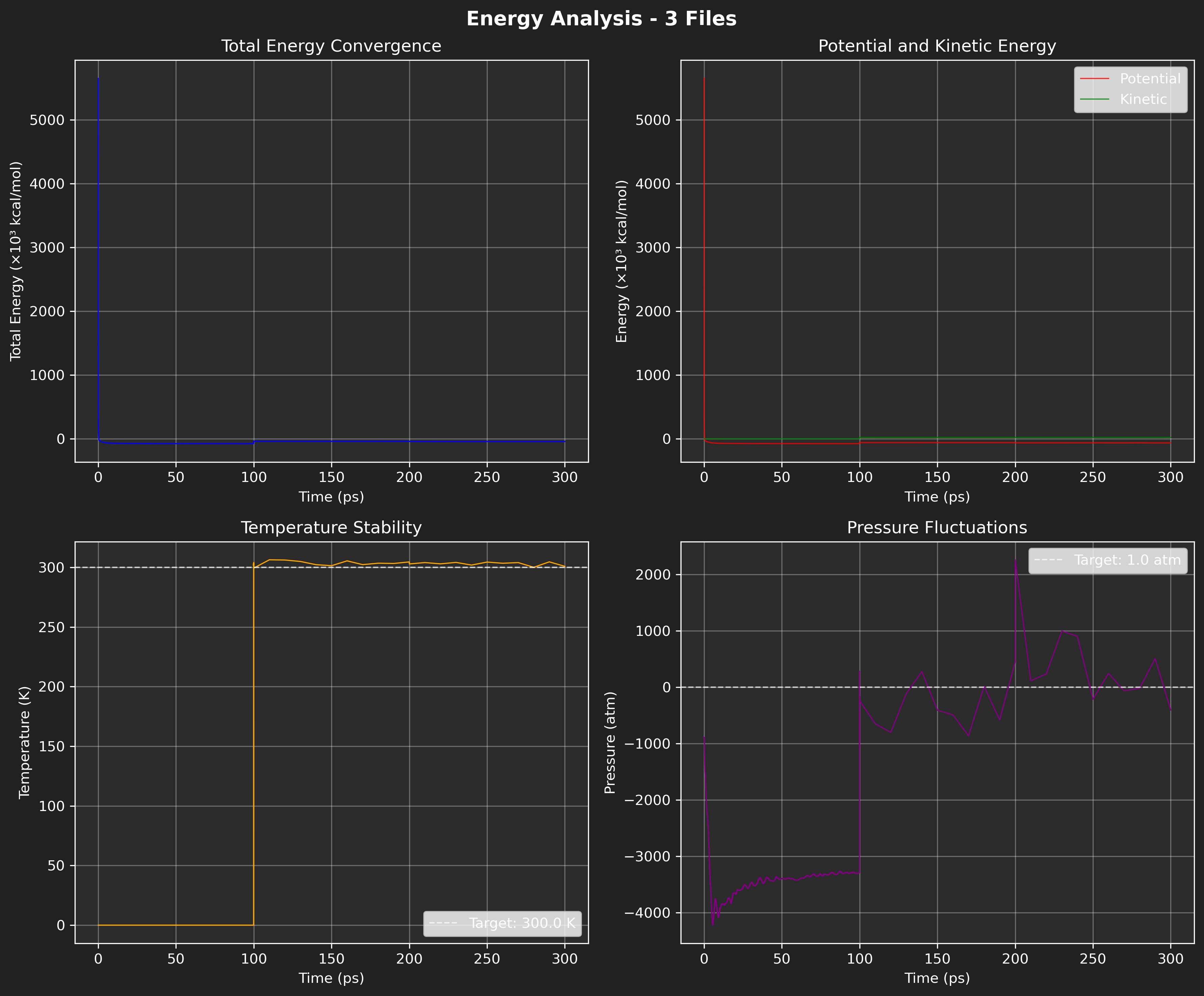
Figure: Default energy plot using the specified NAMD .log files.
Multi-File Color Assignment:
When plotting multiple files on the same plot, colors are automatically assigned:
- If
line_colorsis a single color: all files use that color - If
line_colorsis a list: each file gets corresponding color - If
line_colors=None: auto-assigned from matplotlib color cycle
Time Scaling with file_times:
The file_times parameter in the constructor allows mapping data points to correct time ranges:
# Example: 3 files with different simulation times
# File 1: 0-50 ns (5000 frames)
# File 2: 50-125 ns (7500 frames)
# File 3: 125-200 ns (7500 frames)

analyzer = EnergyAnalyzer(
    log_file=["file1.log", "file2.log", "file3.log"],
    file_times=[(0, 50), (50, 125), (125, 200)],
    # or
    #file_times={
    #    "file1.log": 0.05,  # 50 ps = 0.05 ns
    #    "file2.log": 0.05,
    #    "file3.log": 0.05
    #}
)

# Now time axis will correctly show 0-200 ns with proper frame distribution
analyzer.plot_properties(properties="TEMP", time_units="ns")
Method: get_available_properties()
Get list of all plottable properties available in the loaded log file(s).
Returns: List of property names that can be passed to plot_properties()
Example 2: Get available properties
from pathlib import Path
from gatewizard.utils.namd_analysis import EnergyAnalyzer

# Get the directory where this script is located
script_dir = Path(__file__).parent

# Path to log file in equilibration_folder
log_file = script_dir / "equilibration_folder" / "step1_equilibration.log"

# Initialize energy analyzer
analyzer = EnergyAnalyzer(log_file)
props = analyzer.get_available_properties()
print(f"Can plot: {', '.join(props)}")
# Output: Can plot: Total Energy, Potential Energy, Kinetic Energy,
# Electrostatic Energy, Van der Waals Energy, Bond Energy,
# Angle Energy, Dihedral Energy, Improper Energy, Pressure, Volume
Example 3: Individual energy plots
from pathlib import Path
from gatewizard.utils.namd_analysis import EnergyAnalyzer

# Get the directory where this script is located
script_dir = Path(__file__).parent
data_dir = script_dir / "equilibration_folder"

# Multiple log files from equilibration_folder
log_files = [
    data_dir / "step1_equilibration.log",
    data_dir / "step2_equilibration.log",
    data_dir / "step3_equilibration.log",
    data_dir / "step4_equilibration.log",
    data_dir / "step5_equilibration.log",
    data_dir / "step6_equilibration.log",
    data_dir / "step7_production.log"
]

# Initialize analyzer with custom time for each file (in nanoseconds)
analyzer = EnergyAnalyzer(
    [str(f) for f in log_files],
    file_times={
        "step1_equilibration.log": 0.1,  # 100 ps
        "step2_equilibration.log": 0.1,  # 100 ps
        "step3_equilibration.log": 0.1,  # 100 ps
        "step4_equilibration.log": 0.1,  # 100 ps
        "step5_equilibration.log": 0.1,  # 100 ps
        "step6_equilibration.log": 0.1,  # 100 ps
        "step7_production.log": 0.1,     # 100 ps
    }
)

# Plot specific energy properties
analyzer.plot_properties(
    properties=["bond energy", "angle energy", "dihedral energy"],
    energy_units="kcal/mol",
    time_units="ps",
    bg_color = "#ffffff",
    fig_bg_color = "#FFFFFF",
    save="energy_analysis_example_03.png",
    dpi=300,
)

print(f"Energy properties plot complete!")
print(f"Plot saved: energy_analysis_example_03.png")
Example Output:

Figure: Multiple energy properties plot.
Method: get_statistics()
Get statistical summary of all energy components.
Returns: Dictionary with statistics for each energy term
Statistics Provided:
mean- Average valuestd- Standard deviationmin- Minimum valuemax- Maximum valueinitial- First valuefinal- Last value
Available Energy Terms:
timestep,total,kinetic,potentialelect,vdw,boundary,misctemp,pressure,volume
Example 4: Individual energy plots
from pathlib import Path
from gatewizard.utils.namd_analysis import EnergyAnalyzer

# Get the directory where this script is located
script_dir = Path(__file__).parent

# Path to log file in equilibration_folder
log_file = script_dir / "equilibration_folder" / "step2_equilibration.log"

# Initialize energy analyzer
analyzer = EnergyAnalyzer(log_file)

stats = analyzer.get_statistics()

# Temperature
temp = stats['temp']
print(f"Temperature: {temp['mean']:.1f} ± {temp['std']:.1f} K")
print(f"  Range: {temp['min']:.1f} - {temp['max']:.1f} K")

# Energy
energy = stats['bond']
print(f"Bond Energy: {energy['mean']:.0f} kcal/mol")
print(f"  Final: {energy['final']:.0f} kcal/mol")
print(f"  Convergence: {abs(energy['final'] - energy['mean']):.0f} kcal/mol")

# Output:
# Temperature: 303.6 ± 2.1 K
#   Range: 299.4 - 306.3 K
# Bond Energy: 2080 kcal/mol
#   Final: 2097 kcal/mol
#   Convergence: 17 kcal/mol
Class: TrajectoryAnalyzer
Easy-to-use wrapper for MD trajectory analysis with built-in plotting and full customization.
Constructor
TrajectoryAnalyzer(
    topology: Path,
    trajectory: Path | List[Path],
    file_times: Optional[Dict[str, float]] = None
)
Initialize trajectory analyzer with topology and trajectory file(s).
Parameters:
topology(Path or str): Path to topology file (PSF, PDB, IMPCRD, etc.)trajectory(Path, str, or List): Path(s) to trajectory file(s) (DCD, XTC, TRR, etc.)- Single file:
"trajectory.dcd" - Multiple files:
["eq1.dcd", "eq2.dcd", "prod.dcd"] file_times(Dict[str, float], optional): Mapping of trajectory filenames to their simulation durations in nanoseconds
Example: {"eq1.dcd": 0.05, "eq2.dcd": 0.05, "prod.dcd": 0.05}
- Important: Use just the filename (not full path) as the key
- Time is the duration of that file, not cumulative
- Note: In the GUI, you can input times for each file directly in the file list
Examples:
Single Trajectory:
Multiple Trajectories with Time Scaling:
analyzer = TrajectoryAnalyzer(
    "system.pdb",
    ["step1_equilibration.dcd", "step2_equilibration.dcd", "step7_production.dcd"],
    file_times={
        "step1_equilibration.dcd": 0.05,  # 50 ps
        "step2_equilibration.dcd": 0.05,  # 50 ps
        "step7_production.dcd": 0.05      # 50 ps
    }
)
# Time axis will be continuous: [0...0.05] [0.05...0.10] [0.10...0.15] ns
Method: calculate_rmsd()
Calculate RMSD for selected atoms.
calculate_rmsd(
    selection: str = "protein and backbone",
    reference_frame: int = 0,
    align: bool = True
) -> Dict[str, np.ndarray]
Parameters:
selection(str): MDTraj selection stringreference_frame(int): Frame to use as reference (0 = first frame)align(bool): If True, perform structural alignment (rotation + translation) before RMSD. If False, calculate raw coordinate RMSD without alignment.
Returns: Dictionary with:
'time': Time array in nanoseconds'rmsd': RMSD values in Angstroms
Example:
data = analyzer.calculate_rmsd("protein and backbone", align=True)
print(f"Time range: {data['time'][0]:.3f} - {data['time'][-1]:.3f} ns")
print(f"RMSD range: {data['rmsd'].min():.2f} - {data['rmsd'].max():.2f} Å")
Method: plot_rmsd()
Plot RMSD with full customization options including line styling, threshold highlighting, and convergence line control.
plot_rmsd(
    selection: str = "protein and backbone",
    reference_frame: int = 0,
    align: bool = True,
    distance_units: str = "Å",
    time_units: str = "ns",
    line_color: str = "blue",
    line_width: float = 1.2,
    line_style: str = "-",
    bg_color: str = "#2b2b2b",
    fig_bg_color: str = "#212121",
    text_color: str = "Auto",
    show_grid: bool = True,
    xlim: Optional[tuple] = None,
    ylim: Optional[tuple] = None,
    title: Optional[str] = None,
    xlabel: Optional[str] = None,
    ylabel: Optional[str] = None,
    highlight_threshold: Optional[float] = None,
    highlight_color: str = "orange",
    highlight_alpha: float = 0.2,
    show_convergence: bool = True,
    convergence_color: str = "red",
    convergence_style: str = "--",
    convergence_width: float = 1.5,
    hlines: Optional[List[float]] = None,
    hline_colors: Optional[List[str]] = None,
    hline_styles: Optional[List[str]] = None,
    hline_widths: Optional[List[float]] = None,
    vlines: Optional[List[float]] = None,
    vline_colors: Optional[List[str]] = None,
    vline_styles: Optional[List[str]] = None,
    vline_widths: Optional[List[float]] = None,
    save: Optional[str] = None,
    show: bool = False,
    figsize: tuple = (10, 6),
    dpi: int = 300
)
Parameters:
| Parameter | Type | Default | Description |
|---|---|---|---|
selection | str | "protein and backbone" | MDTraj selection string |
reference_frame | int | 0 | Reference frame index |
align | bool | True | Perform structural alignment before RMSD |
distance_units | str | "Å" | Distance units: "Å" or "nm" |
time_units | str | "ns" | Time units: "ps", "ns", or "µs" |
line_color | str | "blue" | Plot line color (matplotlib color or hex) |
line_width | float | 1.2 | Line thickness/width |
line_style | str | "-" | Line style: "-" (solid), "--" (dashed), "-." (dash-dot), ":" (dotted) |
bg_color | str | "#2b2b2b" | Plot area background (hex or "none") |
fig_bg_color | str | "#212121" | Figure border background (hex or "none") |
text_color | str | "Auto" | Text/axes color ("Auto", color, or hex) |
show_grid | bool | True | Show grid lines |
xlim | tuple or None | None | X-axis limits (min, max) |
ylim | tuple or None | None | Y-axis limits (min, max) |
title | str or None | None | Custom title (auto-generated if None) |
xlabel | str or None | None | Custom X-label (auto with units if None) |
ylabel | str or None | None | Custom Y-label (auto with units if None) |
highlight_threshold | float or None | None | Highlight regions above this RMSD value |
highlight_color | str | "orange" | Color for highlight region and line |
highlight_alpha | float | 0.2 | Alpha transparency for highlight fill |
show_convergence | bool | True | Show convergence line (mean of last 20% of trajectory) |
convergence_color | str | "red" | Color for convergence line |
convergence_style | str | "--" | Line style for convergence line |
convergence_width | float | 1.5 | Width of convergence line |
hlines | list or None | None | List of Y values for horizontal reference lines |
hline_colors | list or None | None | List of colors for horizontal lines |
hline_styles | list or None | None | List of line styles for horizontal lines (default: "--") |
hline_widths | list or None | None | List of line widths for horizontal lines (default: 1.0) |
vlines | list or None | None | List of X values for vertical reference lines |
vline_colors | list or None | None | List of colors for vertical lines |
vline_styles | list or None | None | List of line styles for vertical lines (default: "--") |
vline_widths | list or None | None | List of line widths for vertical lines (default: 1.0) |
save | str or None | None | Filename to save plot |
show | bool | False | Display plot interactively |
figsize | tuple | (10, 6) | Figure size (width, height) |
dpi | int | 300 | Resolution for saved figure |
Example 5: RMSD Plot
from pathlib import Path
from gatewizard.utils.namd_analysis import TrajectoryAnalyzer

# Get the directory where this script is located
script_dir = Path(__file__).parent
data_dir = script_dir / "equilibration_folder"

# Path to topology in equilibration_folder
topology_file = data_dir / "system.pdb"

# Multiple trajectory files from equilibration_folder
trajectory_files = [
    data_dir / "step1_equilibration.dcd",
    data_dir / "step2_equilibration.dcd",
    data_dir / "step3_equilibration.dcd"
]

# Initialize analyzer with custom time for each file (in nanoseconds)
analyzer = TrajectoryAnalyzer(
    topology_file,
    trajectory_files,
    file_times={
        "step1_equilibration.dcd": 0.1,  # 100 ps
        "step2_equilibration.dcd": 0.1,  # 100 ps
        "step3_equilibration.dcd": 0.1   # 100 ps
    }
)

# Plot RMSD across all trajectories
analyzer.plot_rmsd(
    selection="protein and backbone",
    time_units="ns",
    bg_color="white",
    fig_bg_color="white",
    text_color="black",
    show_grid=False,
    line_color="#1f77b4",
    line_width=2,
    #title=" ",
    save="trajectory_analysis_example_05.png",
    dpi=300,
    # other settings...
)


print(f"Multi-file trajectory analysis complete!")
print(f"Plot saved: trajectory_analysis_example_05.png")
print(f"Total simulation time: 300 ps")
Method: calculate_rmsf()
Calculate RMSF (Root Mean Square Fluctuation) for selected atoms.
Parameters:
selection(str): MDTraj selection string
Returns: Dictionary with:
'resids': Residue numbers'rmsf': RMSF values in Angstroms'resnames': Residue names (e.g., ALA, GLY, VAL)'atom_indices': Atom indices
Example 6: RMSF Calculation
from pathlib import Path
from gatewizard.utils.namd_analysis import TrajectoryAnalyzer

# Get the directory where this script is located
script_dir = Path(__file__).parent
data_dir = script_dir / "equilibration_folder"

# Path to topology in equilibration_folder
topology_file = data_dir / "system.pdb"

# Multiple trajectory files from equilibration_folder
trajectory_files = [
    data_dir / "step1_equilibration.dcd",
    data_dir / "step2_equilibration.dcd",
    data_dir / "step3_equilibration.dcd"
]

# Initialize analyzer with custom time for each file (in nanoseconds)
analyzer = TrajectoryAnalyzer(
    topology_file,
    trajectory_files,
    file_times={
        "step1_equilibration.dcd": 0.1,  # 100 ps
        "step2_equilibration.dcd": 0.1,  # 100 ps
        "step3_equilibration.dcd": 0.1   # 100 ps
    }
)

# Calculate RMSF for alpha carbon atoms
data = analyzer.calculate_rmsf("protein and name CA")
print(f"Residues analyzed: {len(data['resids'])}")
print(f"RMSF range: {data['rmsf'].min():.2f} - {data['rmsf'].max():.2f} Å")
print(f"Mean RMSF: {data['rmsf'].mean():.2f} Å")

# Output:
# Residues analyzed: 26
# RMSF range: 0.09 - 0.15 Å
# Mean RMSF: 0.12 Å
Method: plot_rmsf()
Plot RMSF with full customization including line styling, residue labeling, and flexibility highlighting.
plot_rmsf(
    selection: str = "protein and name CA",
    xaxis_type: str = "residue_number",
    show_residue_labels: bool = True,
    residue_name_format: str = "single",
    label_frequency: str = "auto",
    distance_units: str = "Å",
    line_color: str = "blue",
    line_width: float = 1.2,
    line_style: str = "-",
    bg_color: str = "#2b2b2b",
    fig_bg_color: str = "#212121",
    text_color: str = "Auto",
    show_grid: bool = True,
    xlim: Optional[tuple] = None,
    ylim: Optional[tuple] = None,
    title: Optional[str] = None,
    xlabel: Optional[str] = None,
    ylabel: Optional[str] = None,
    highlight_threshold: Optional[float] = None,
    highlight_color: str = "orange",
    highlight_alpha: float = 0.2,
    hlines: Optional[List[float]] = None,
    hline_colors: Optional[List[str]] = None,
    hline_styles: Optional[List[str]] = None,
    hline_widths: Optional[List[float]] = None,
    vlines: Optional[List[float]] = None,
    vline_colors: Optional[List[str]] = None,
    vline_styles: Optional[List[str]] = None,
    vline_widths: Optional[List[float]] = None,
    save: Optional[str] = None,
    show: bool = False,
    figsize: tuple = (12, 6),
    dpi: int = 300
)
Parameters:
| Parameter | Type | Default | Description |
|---|---|---|---|
selection | str | "protein and name CA" | MDTraj selection string |
xaxis_type | str | "residue_number" | X-axis type: "residue_number", "residue_type_number", "atom_index" |
show_residue_labels | bool | True | Show residue labels on X-axis |
residue_name_format | str | "single" | Residue format: "single" (A, G, V) or "triple" (ALA, GLY, VAL) |
label_frequency | str | "auto" | Label frequency: "all", "auto", "every_2", "every_5", "every_10", "every_20" |
distance_units | str | "Å" | Distance units: "Å" or "nm" |
line_color | str | "blue" | Plot line color (matplotlib color or hex) |
line_width | float | 1.2 | Line thickness/width |
line_style | str | "-" | Line style: "-" (solid), "--" (dashed), "-." (dash-dot), ":" (dotted) |
highlight_threshold | float or None | None | If set, highlight residues above this RMSF value |
highlight_color | str | "orange" | Color for highlight region and threshold line |
highlight_alpha | float | 0.2 | Alpha transparency for highlight fill region |
hlines | list or None | None | List of Y values for horizontal reference lines |
hline_colors | list or None | None | List of colors for horizontal lines (cycles if fewer than lines) |
hline_styles | list or None | None | List of line styles for horizontal lines (default: "--") |
hline_widths | list or None | None | List of line widths for horizontal lines (default: 1.0) |
vlines | list or None | None | List of X values (residue numbers) for vertical reference lines |
vline_colors | list or None | None | List of colors for vertical lines (cycles if fewer than lines) |
vline_styles | list or None | None | List of line styles for vertical lines (default: "--") |
vline_widths | list or None | None | List of line widths for vertical lines (default: 1.0) |
| ...other params | Same as plot_rmsd() for colors, grid, limits, etc. |
X-Axis Types:
"residue_number"- Simple numbers: 1, 2, 3, ..."residue_type_number"- Type + number: ALA1, GLY2, VAL3, ..."atom_index"- Atom indices: 0, 15, 30, ...
Label Frequencies:
"all"- Every residue labeled"auto"- Smart frequency based on count (<20: all, <50: every_2, <100: every_5, <200: every_10, else: every_20)"every_2","every_5","every_10","every_20"- Specific intervals
Example 7: RMSF Plotting
from pathlib import Path
from gatewizard.utils.namd_analysis import TrajectoryAnalyzer

# Get the directory where this script is located
script_dir = Path(__file__).parent
data_dir = script_dir / "equilibration_folder"

# Path to topology in equilibration_folder
topology_file = data_dir / "system.pdb"

# Multiple trajectory files from equilibration_folder
trajectory_files = [
    data_dir / "step1_equilibration.dcd",
    data_dir / "step2_equilibration.dcd",
    data_dir / "step3_equilibration.dcd",
    data_dir / "step4_equilibration.dcd",
    data_dir / "step5_equilibration.dcd",
    data_dir / "step6_equilibration.dcd",
    data_dir / "step7_production.dcd",
]

# Initialize analyzer with custom time for each file (in nanoseconds)
analyzer = TrajectoryAnalyzer(
    topology_file,
    trajectory_files,
    file_times={
        "step1_equilibration.dcd": 0.1,  # 100 ps
        "step2_equilibration.dcd": 0.1,  # 100 ps
        "step3_equilibration.dcd": 0.1,   # 100 ps
        "step4_equilibration.dcd": 0.1,  # 100 ps
        "step5_equilibration.dcd": 0.1,  # 100 ps
        "step6_equilibration.dcd": 0.1,  # 100 ps
        "step7_production.dcd": 0.1      # 100 ps
    }
)

# Plot RMSF across all trajectories
analyzer.plot_rmsf(
    selection="protein and name C",
    xaxis_type= "residue_type_number",
    residue_name_format="triple",
    label_frequency="all",
    highlight_threshold=0.6,
    highlight_color="red",
    bg_color="white",
    fig_bg_color="white",
    text_color="black",
    show_grid=False,
    line_color="#1f77b4",
    line_width=2,
    #title=" ",
    save="trajectory_analysis_example_07.png",
    dpi=300,
    # other settings...
)
Output figure:
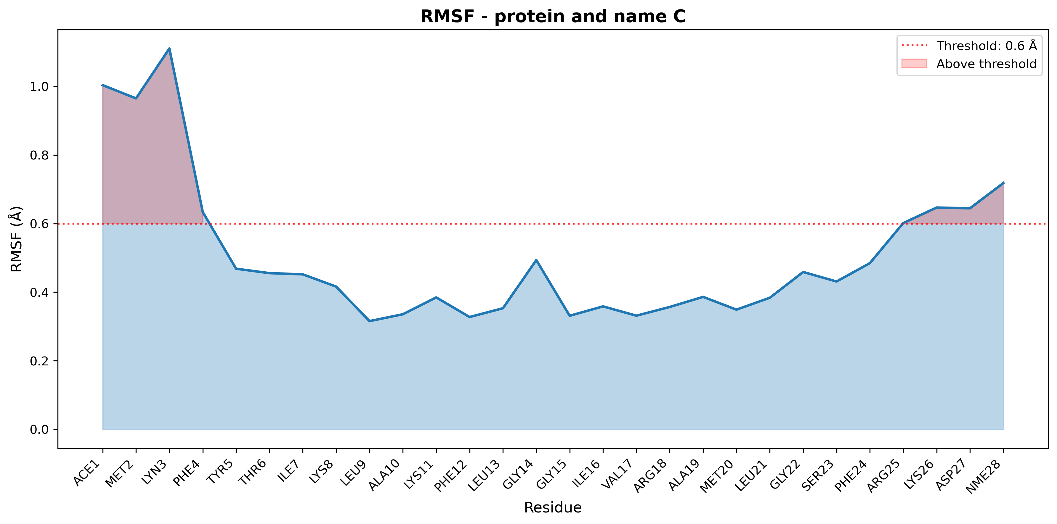
Figure: RMSF plot for multiple with threshold highlight.
Method: calculate_distances()
Calculate distances between atom selections over time.
Parameters:
selections(dict): Dictionary of{name: (selection1, selection2)}
Returns: Dictionary with distance data for each named selection:
'time': Time array in nanoseconds'distance': Distance array in Angstroms
Example:
results = analyzer.calculate_distances({
    "gate": ("resid 1-3 and name CA", "resid 18-20 and name CA"),
    "binding_site": ("resid 100-110", "resname LIG")
})

for name, data in results.items():
    print(f"{name}:")
    print(f"  Time: {data['time'][0]:.3f} - {data['time'][-1]:.3f} ns")
    print(f"  Distance: {data['distance'].mean():.2f} ± {data['distance'].std():.2f} Å")
Method: plot_distances()
Plot distances with full customization including line styling.
plot_distances(
    selections: Dict[str, tuple],
    distance_units: str = "Å",
    time_units: str = "ns",
    line_colors: Optional[List[str]] = None,
    line_width: float = 1.2,
    line_style: str = "-",
    bg_color: str = "#2b2b2b",
    fig_bg_color: str = "#212121",
    text_color: str = "Auto",
    show_grid: bool = True,
    xlim: Optional[tuple] = None,
    ylim: Optional[tuple] = None,
    title: Optional[str] = None,
    xlabel: Optional[str] = None,
    ylabel: Optional[str] = None,
    show_mean_lines: bool = True,
    hlines: Optional[List[float]] = None,
    hline_colors: Optional[List[str]] = None,
    hline_styles: Optional[List[str]] = None,
    hline_widths: Optional[List[float]] = None,
    vlines: Optional[List[float]] = None,
    vline_colors: Optional[List[str]] = None,
    vline_styles: Optional[List[str]] = None,
    vline_widths: Optional[List[float]] = None,
    save: Optional[str] = None,
    show: bool = False,
    figsize: tuple = (10, 6),
    dpi: int = 300
)
Parameters:
| Parameter | Type | Default | Description |
|---|---|---|---|
selections | dict | - | Dictionary of {name: (sel1, sel2)} |
distance_units | str | "Å" | Distance units: "Å" or "nm" |
time_units | str | "ns" | Time units: "ps", "ns", or "µs" |
line_colors | list or None | None | List of colors for each distance pair |
line_width | float | 1.2 | Line thickness/width |
line_style | str | "-" | Line style: "-" (solid), "--" (dashed), "-." (dash-dot), ":" (dotted) |
show_mean_lines | bool | True | Show dashed mean distance lines |
hlines | list or None | None | List of Y values for horizontal reference lines |
hline_colors | list or None | None | List of colors for horizontal lines (cycles if fewer than lines) |
hline_styles | list or None | None | List of line styles for horizontal lines (default: "--") |
hline_widths | list or None | None | List of line widths for horizontal lines (default: 1.0) |
vlines | list or None | None | List of X values (time points) for vertical reference lines |
vline_colors | list or None | None | List of colors for vertical lines (cycles if fewer than lines) |
vline_styles | list or None | None | List of line styles for vertical lines (default: "--") |
vline_widths | list or None | None | List of line widths for vertical lines (default: 1.0) |
| ...other params | Same as plot_rmsd() |
Example 8: Distances
from pathlib import Path
from gatewizard.utils.namd_analysis import TrajectoryAnalyzer

# Get the directory where this script is located
script_dir = Path(__file__).parent
data_dir = script_dir / "equilibration_folder"

# Path to topology in equilibration_folder
topology_file = data_dir / "system.pdb"

# Multiple trajectory files from equilibration_folder
trajectory_files = [
    data_dir / "step1_equilibration.dcd",
    data_dir / "step2_equilibration.dcd",
    data_dir / "step3_equilibration.dcd",
    data_dir / "step4_equilibration.dcd",
    data_dir / "step5_equilibration.dcd",
    data_dir / "step6_equilibration.dcd",
    data_dir / "step7_production.dcd",
]

# Initialize analyzer with custom time for each file (in nanoseconds)
analyzer = TrajectoryAnalyzer(
    topology_file,
    trajectory_files,
    file_times={
        "step1_equilibration.dcd": 0.1,  # 100 ps
        "step2_equilibration.dcd": 0.1,  # 100 ps
        "step3_equilibration.dcd": 0.1,   # 100 ps
        "step4_equilibration.dcd": 0.1,  # 100 ps
        "step5_equilibration.dcd": 0.1,  # 100 ps
        "step6_equilibration.dcd": 0.1,  # 100 ps
        "step7_production.dcd": 0.1      # 100 ps
    }
)
# Calculate and plot distances between selections
analyzer.plot_distances(
    selections={
        "gate_distance": ("resid 1 and name C", "resid 28 and name C"),
        "domain_distance": ("resid 1-2 and name C", "resid 9-10 and name C")
    },
    bg_color="white",
    fig_bg_color="white",
    text_color="black",
    line_width=3,
    save="trajectory_analysis_example_08_distances.png"
)

print(f"Distances plot saved: trajectory_analysis_example_08_distances.png")
Output figure:
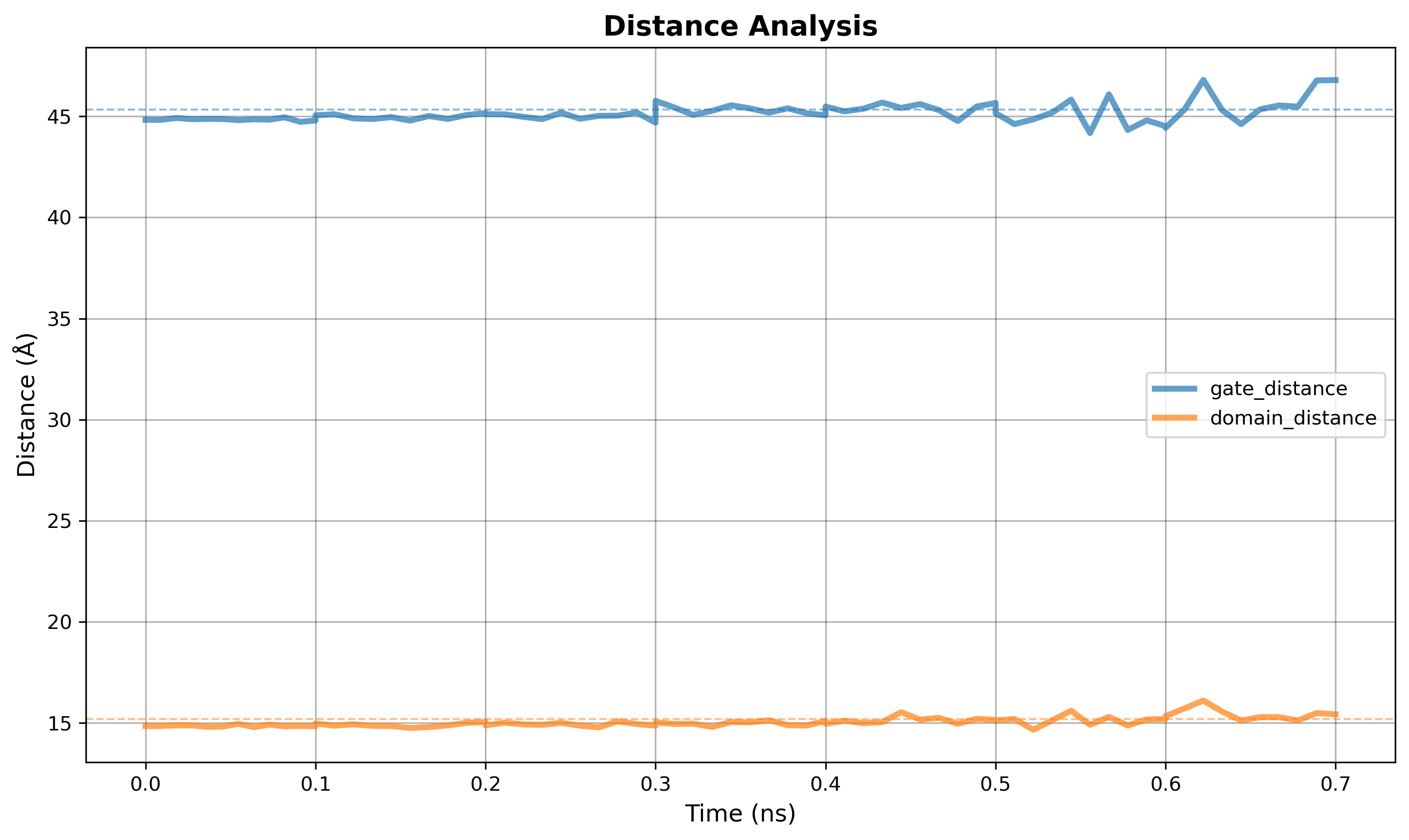
Figure: Distances plot for multiple defined regions on the protein.
Method: calculate_radius_of_gyration()
Calculate radius of gyration over trajectory.
Parameters:
selection(str): MDTraj selection string
Returns: Dictionary with:
'time': Time array in nanoseconds'rg': Radius of gyration in Angstroms
Example:
data = analyzer.calculate_radius_of_gyration("protein")
print(f"Rg range: {data['rg'].min():.2f} - {data['rg'].max():.2f} Å")
print(f"Mean Rg: {data['rg'].mean():.2f} Å")
Method: plot_radius_of_gyration()
Plot radius of gyration with full customization including line styling and convergence control.
plot_radius_of_gyration(
    selection: str = "protein",
    distance_units: str = "Å",
    time_units: str = "ns",
    line_color: str = "purple",
    line_width: float = 1.2,
    line_style: str = "-",
    bg_color: str = "#2b2b2b",
    fig_bg_color: str = "#212121",
    text_color: str = "Auto",
    show_grid: bool = True,
    xlim: Optional[tuple] = None,
    ylim: Optional[tuple] = None,
    title: Optional[str] = None,
    xlabel: Optional[str] = None,
    ylabel: Optional[str] = None,
    show_convergence: bool = True,
    convergence_color: str = "red",
    convergence_style: str = "--",
    convergence_width: float = 1.5,
    hlines: Optional[List[float]] = None,
    hline_colors: Optional[List[str]] = None,
    hline_styles: Optional[List[str]] = None,
    hline_widths: Optional[List[float]] = None,
    vlines: Optional[List[float]] = None,
    vline_colors: Optional[List[str]] = None,
    vline_styles: Optional[List[str]] = None,
    vline_widths: Optional[List[float]] = None,
    save: Optional[str] = None,
    show: bool = False,
    figsize: tuple = (10, 6),
    dpi: int = 300
)
Parameters:
| Parameter | Type | Default | Description |
|---|---|---|---|
selection | str | "protein" | MDTraj selection string |
distance_units | str | "Å" | Distance units: "Å" or "nm" |
time_units | str | "ns" | Time units: "ps", "ns", or "µs" |
line_color | str | "purple" | Plot line color (matplotlib color or hex) |
line_width | float | 1.2 | Line thickness/width |
line_style | str | "-" | Line style: "-" (solid), "--" (dashed), "-." (dash-dot), ":" (dotted) |
show_convergence | bool | True | Show convergence line (mean of last 20% of trajectory) |
convergence_color | str | "red" | Color for convergence line |
convergence_style | str | "--" | Line style for convergence line |
convergence_width | float | 1.5 | Width of convergence line |
hlines | list or None | None | List of Y values for horizontal reference lines |
hline_colors | list or None | None | List of colors for horizontal lines (cycles if fewer than lines) |
hline_styles | list or None | None | List of line styles for horizontal lines (default: "--") |
hline_widths | list or None | None | List of line widths for horizontal lines (default: 1.0) |
vlines | list or None | None | List of X values (time points) for vertical reference lines |
vline_colors | list or None | None | List of colors for vertical lines (cycles if fewer than lines) |
vline_styles | list or None | None | List of line styles for vertical lines (default: "--") |
vline_widths | list or None | None | List of line widths for vertical lines (default: 1.0) |
| ...other params | Same as plot_rmsd() for colors, grid, limits, etc. |
Example 9: Radius of gyration
from pathlib import Path
from gatewizard.utils.namd_analysis import TrajectoryAnalyzer

# Get the directory where this script is located
script_dir = Path(__file__).parent
data_dir = script_dir / "equilibration_folder"

# Path to topology in equilibration_folder
topology_file = data_dir / "system.pdb"

# Multiple trajectory files from equilibration_folder
trajectory_files = [
    data_dir / "step1_equilibration.dcd",
    data_dir / "step2_equilibration.dcd",
    data_dir / "step3_equilibration.dcd",
    data_dir / "step4_equilibration.dcd",
    data_dir / "step5_equilibration.dcd",
    data_dir / "step6_equilibration.dcd",
    data_dir / "step7_production.dcd",
]

# Initialize analyzer with custom time for each file (in nanoseconds)
analyzer = TrajectoryAnalyzer(
    topology_file,
    trajectory_files,
    file_times={
        "step1_equilibration.dcd": 0.1,  # 100 ps
        "step2_equilibration.dcd": 0.1,  # 100 ps
        "step3_equilibration.dcd": 0.1,   # 100 ps
        "step4_equilibration.dcd": 0.1,  # 100 ps
        "step5_equilibration.dcd": 0.1,  # 100 ps
        "step6_equilibration.dcd": 0.1,  # 100 ps
        "step7_production.dcd": 0.1      # 100 ps
    }
)
# Calculate and plot radius of gyration of a selection
analyzer.plot_radius_of_gyration(
    selection="protein",
    bg_color="white",
    fig_bg_color="white",
    text_color="black",
    line_width=3,
    save="trajectory_analysis_example_09_rdgyr.png",
    dpi=300,
)
Method: plot_comprehensive()
Create a 4-panel analysis plot with RMSD, RMSF, Rg, and statistics.
plot_comprehensive(
    save: Optional[str] = None,
    show: bool = False,
    figsize: tuple = (14, 10),
    dpi: int = 300
)
Parameters:
save(str, optional): Filename to save plotshow(bool): Display plot interactivelyfigsize(tuple): Figure sizedpi(int): Resolution
Example:
Tips & Best Practices
1. Always Provide file_times for Multiple Files
# ✅ GOOD: Proper time scaling
file_times = {
    "step1_equilibration.dcd": 0.05,  # 50 ps
    "step2_equilibration.dcd": 0.05,
    "step3_equilibration.dcd": 0.05
}

# ❌ BAD: Frame-based time (incorrect)
file_times = None  # Will use frame indices
2. Match Units to Your Analysis
# Short simulations (< 1 ns)
time_units="ps", distance_units="Å"

# Medium simulations (1-100 ns)
time_units="ns", distance_units="Å"

# Long simulations (> 100 ns)
time_units="ns", distance_units="nm"
3. RMSF Labeling for Different Protein Sizes
# Small protein (< 100 residues)
label_frequency="every_2"

# Medium protein (100-300 residues)
label_frequency="every_5"

# Large protein (> 300 residues)
label_frequency="every_10" or "every_20"
4. Color Schemes
# Dark theme (presentations)
bg_color="#2b2b2b", text_color="Auto"

# Light theme (publications)
bg_color="#ffffff", text_color="black"

# Transparent (overlays)
bg_color="none", fig_bg_color="none"
Function: get_equilibration_progress()
Get progress information from NAMD equilibration logs.
get_equilibration_progress(
    log_directory: Path,
    output_file: Optional[Path] = None
) -> Dict[str, NAMDProgress]
Parameters:
log_directory(Path): Directory containing NAMD log filesoutput_file(Path, optional): Save progress summary to JSON
Returns: Dictionary of progress information for each stage
Example:
from gatewizard.utils.namd_analysis import get_equilibration_progress

progress = get_equilibration_progress("equilibration/")
for stage, info in progress.items():
    print(f"{stage}: {info.progress_percent:.1f}% complete")
Line Styling and Customization
All trajectory analysis plotting methods (plot_rmsd(), plot_rmsf(), plot_distances(), plot_radius_of_gyration()) support line styling options for full control over plot appearance.
Common Line Parameters
Available in all plotting methods:
| Parameter | Type | Default | Description |
|---|---|---|---|
line_color | str | varies | Color name (e.g., "blue") or hex code (e.g., "#1f77b4") |
line_width | float | 1.2 | Line thickness (e.g., 0.8, 1.5, 2.5) |
line_style | str | "-" | Line style (see options below) |
Line Style Options
| Style | Value | Visual | Use Case |
|---|---|---|---|
| Solid | "-" | ──────── | Default, standard plots |
| Dashed | "--" | ── ── ── | Highlighting, predictions |
| Dash-dot | "-." | ── · ── · | Alternative highlighting |
| Dotted | ":" | · · · · · | Subtle lines, backgrounds |
RMSD & Radius of Gyration Specific
Additional convergence line control for plot_rmsd() and plot_radius_of_gyration():
| Parameter | Type | Default | Description |
|---|---|---|---|
show_convergence | bool | True | Toggle convergence line on/off |
convergence_color | str | "red" | Color for convergence line |
convergence_style | str | "--" | Line style for convergence |
convergence_width | float | 1.5 | Width of convergence line |
RMSD Specific
Threshold highlighting for plot_rmsd():
| Parameter | Type | Default | Description |
|---|---|---|---|
highlight_threshold | float or None | None | Highlight regions above this RMSD value (in Å or nm) |
RMSF Specific
Flexibility highlighting for plot_rmsf():
| Parameter | Type | Default | Description |
|---|---|---|---|
highlight_threshold | float or None | None | Highlight residues above this RMSF value (in Å or nm) |
Quick Reference Examples
Thick Dashed Line:
Thin Dotted Line:
Custom Convergence (Green Dash-dot):
No Convergence Line:
RMSD with Threshold:
RMSF with Flexibility Threshold:
MDTraj Selection Syntax
Common Selections
"protein"                          # All protein atoms
"protein and backbone"             # Backbone atoms (N, CA, C, O)
"protein and name CA"              # C-alpha atoms only
"resid 50-150"                     # Residues 50 to 150
"resid 50-70 and name CA"          # C-alpha of residues 50-70
"resname LIG"                      # Ligand with residue name LIG
"protein and not name H*"          # Protein without hydrogens
"within 5 of resname LIG"          # Atoms within 5Å of ligand
Combining Selections
"(resid 1-50) or (resid 100-150)"    # Two regions
"protein and (name CA or name N)"    # Multiple atom names
"resid 25 and name NH1 NH2"          # Multiple atoms in residue
Class: BilayerTrajectoryAnalyzer
Lipid bilayer analysis built on lipyphilic and MDAnalysis.
Constructor
BilayerTrajectoryAnalyzer(
    topology: Path,
    trajectory: Path | List[Path],
    file_times: Optional[Dict[str, float]] = None
)
Same topology/trajectory interface as TrajectoryAnalyzer. Leaflet assignment is performed automatically before each analysis.
Method: calculate_area_per_lipid()
Calculate the area per lipid via 2D Voronoi tessellation (lipyphilic AreaPerLipid).
calculate_area_per_lipid(
    lipid_sel: str = "name PO4",
    leaflet_lipid_sel: Optional[str] = None,
    start: Optional[int] = None,
    stop: Optional[int] = None,
    step: Optional[int] = None,
    verbose: bool = False,
) -> Dict[str, np.ndarray]
Parameters:
| Parameter | Description |
|---|---|
lipid_sel | Atoms used for Voronoi tessellation. MARTINI: "name GL1 GL2 ROH". All-atom: "name PO4" or phosphate selections. |
leaflet_lipid_sel | Selection for leaflet assignment. Defaults to lipid_sel. |
start, stop, step | Trajectory frame range passed to lipyphilic. |
Returns: time (ns), areas (n_lipids × n_frames, Ų), mean_area_per_lipid, mean_upper_leaflet, mean_lower_leaflet, resids, resnames.
See Example 14: Area per Lipid.
Method: calculate_membrane_thickness()
Calculate bilayer thickness from interleaflet headgroup distances (lipyphilic MembThickness).
calculate_membrane_thickness(
    lipid_sel: str = "name PO4",
    leaflet_lipid_sel: Optional[str] = None,
    leaflet_filter_sel: Optional[str] = None,
    n_bins: int = 1,
    interpolate: bool = False,
    start: Optional[int] = None,
    stop: Optional[int] = None,
    step: Optional[int] = None,
    verbose: bool = False,
) -> Dict[str, np.ndarray]
Parameters:
| Parameter | Description |
|---|---|
lipid_sel | Headgroup atoms for the thickness calculation. |
leaflet_lipid_sel | Selection for leaflet assignment. Defaults to lipid_sel. |
leaflet_filter_sel | Optional filter passed to AssignLeaflets.filter_leaflets() to exclude species (e.g. cholesterol). |
n_bins | Grid resolution for intrinsic surface construction (1 = global mean height). |
interpolate | Fill missing grid values when n_bins is large (slower). |
Returns: time (ns), thickness (Å).
See Example 15: Membrane Thickness.
Method: plot_area_per_lipid() / plot_membrane_thickness()
Generate time-series plots with the same styling options as TrajectoryAnalyzer plots. See Examples 14 and 15.
Function: run_bilayer_analysis()
JSON-serializable API for GUI and downstream consumers.
run_bilayer_analysis(
    topology_file: Union[str, Path],
    trajectory_files: List[Union[str, Path]],
    analysis_type: str,
    lipid_sel: str = "name PO4",
    leaflet_lipid_sel: Optional[str] = None,
    leaflet_filter_sel: Optional[str] = None,
    n_bins: int = 1,
    interpolate: bool = False,
    file_times: Optional[Dict[str, float]] = None,
    start: Optional[int] = None,
    stop: Optional[int] = None,
    step: Optional[int] = None,
    verbose: bool = False,
) -> Dict[str, Any]
Supported analysis_type values: area_per_lipid, membrane_thickness (aliases: apl, thickness, memb_thickness).
Area per lipid return shape:
{
    "analysis_type": "area_per_lipid",
    "x": [...],           # time (ns)
    "y": [...],           # mean area per lipid (Ų)
    "mean_upper_leaflet": [...],
    "mean_lower_leaflet": [...],
    "lipid_resids": [...],
    "lipid_resnames": [...],
    "per_lipid_areas": [[...], ...],
    "stats": {"mean", "std", "min", "max"},
}
Membrane thickness return shape:
{
    "analysis_type": "membrane_thickness",
    "x": [...],
    "y": [...],           # thickness (Å)
    "n_bins": 1,
    "stats": {"mean", "std", "min", "max"},
}
Examples
Complete working examples are available in Analysis examples. Each example demonstrates specific analysis capabilities and can be run directly.
Example 10: Dark Theme RMSD Analysis - Full Customization
Complete RMSD customization with dark themes showing all available plot options.
from pathlib import Path
from gatewizard.utils.namd_analysis import TrajectoryAnalyzer

# Get the directory where this script is located
script_dir = Path(__file__).parent
data_dir = script_dir / "equilibration_folder"

# ============================================================================
# Dark Theme RMSD Analysis - Full Customization
# ============================================================================

topology_file = data_dir / "system.pdb"
# Multiple trajectory files from equilibration_folder
trajectory_files = [
    data_dir / "step1_equilibration.dcd",
    data_dir / "step2_equilibration.dcd",
    data_dir / "step3_equilibration.dcd",
    data_dir / "step4_equilibration.dcd",
]

# Initialize analyzer with custom time for each file (in nanoseconds)
analyzer = TrajectoryAnalyzer(
    topology_file,
    trajectory_files,
    file_times={
        "step1_equilibration.dcd": 0.1,  # 100 ps
        "step2_equilibration.dcd": 0.1,  # 100 ps
        "step3_equilibration.dcd": 0.1,   # 100 ps
        "step4_equilibration.dcd": 0.1,  # 100 ps
    }
)

# RMSD plot with full dark theme customization
analyzer.plot_rmsd(
    selection="protein and backbone",
    reference_frame=0,
    align=True,
    distance_units="Å",
    time_units="ps",
    line_color="#00d9ff",        # Bright cyan
    line_width=2.0,
    line_style="-",
    bg_color="#1a1a2e",          # Dark blue-black
    fig_bg_color="#16213e",      # Darker border
    text_color="#eee",           # Light gray
    show_grid=True,
    xlim=None,
    ylim=None,
    title="Dark Theme RMSD - Full Customization",
    xlabel="Time (ps)",
    ylabel="RMSD (Å)",
    highlight_threshold=None,
    highlight_color="orange",
    highlight_alpha=0.2,
    show_convergence=True,
    convergence_color="#ff006e",  # Magenta
    convergence_style="--",
    convergence_width=2.0,
    hlines=None,
    hline_colors=None,
    hline_styles=None,
    hline_widths=None,
    vlines=None,
    vline_colors=None,
    vline_styles=None,
    vline_widths=None,
    save="dark_theme_rmsd_example_10.png",
    show=False,
    figsize=(12, 7),
    dpi=300
)

print(f"Dark theme RMSD plot saved: dark_theme_rmsd_example_10.png")

# ============================================================================
# Dark Theme RMSD - With Threshold and Reference Lines
# ============================================================================

analyzer.plot_rmsd(
    selection="protein and backbone",
    align=True,
    distance_units="Å",
    time_units="ps",
    line_color="#7fff00",        # Chartreuse
    line_width=1.8,
    line_style="-",
    bg_color="#0d1117",          # GitHub dark
    fig_bg_color="#010409",
    text_color="#c9d1d9",
    show_grid=True,
    title="Dark Theme RMSD - With Threshold and Reference Lines",
    xlabel="Time (ps)",
    ylabel="RMSD (Å)",
    highlight_threshold=0.25,     # Highlight regions > 0.25 Å
    highlight_color="#ff6b6b",   # Red highlight
    highlight_alpha=0.5,
    show_convergence=True,
    convergence_color="#ffd700",  # Gold
    convergence_style="-.",
    convergence_width=1.5,
    hlines=[0.1, 0.2, 0.25],      # Horizontal reference lines
    hline_colors=["#4ecdc4", "#95e1d3", "#ff6b6b"],  # Teal to red gradient
    hline_styles=[":", ":", ":"],
    hline_widths=[1.0, 1.0, 1.0],
    save="dark_theme_rmsd_with_lines_example_10.png",
    figsize=(12, 7),
    dpi=300
)

print(f"Dark theme RMSD with lines saved: dark_theme_rmsd_with_lines_example_10.png")

# ============================================================================
# Dark Theme RMSD - Minimal Style
# ============================================================================

analyzer.plot_rmsd(
    selection="protein and backbone",
    align=True,
    distance_units="Å",
    time_units="ps",
    line_color="#ffffff",        # Pure white line
    line_width=1.5,
    line_style="-",
    bg_color="#000000",          # Pure black
    fig_bg_color="#000000",
    text_color="#ffffff",
    show_grid=False,             # No grid for minimal look
    title="",                    # No title
    show_convergence=False,      # No convergence line
    save="dark_theme_rmsd_minimal_example_10.png",
    figsize=(10, 6),
    dpi=300
)

print(f"Dark theme RMSD minimal saved: dark_theme_rmsd_minimal_example_10.png")

print(f"\nAll dark theme RMSD figures created with:")
print(f"  - Custom dark backgrounds")
print(f"  - Full customization options")
print(f"  - High resolution (300 DPI)")
Output figures Three dark-themed RMSD plots:
Figure: Dark theme RMSD plot
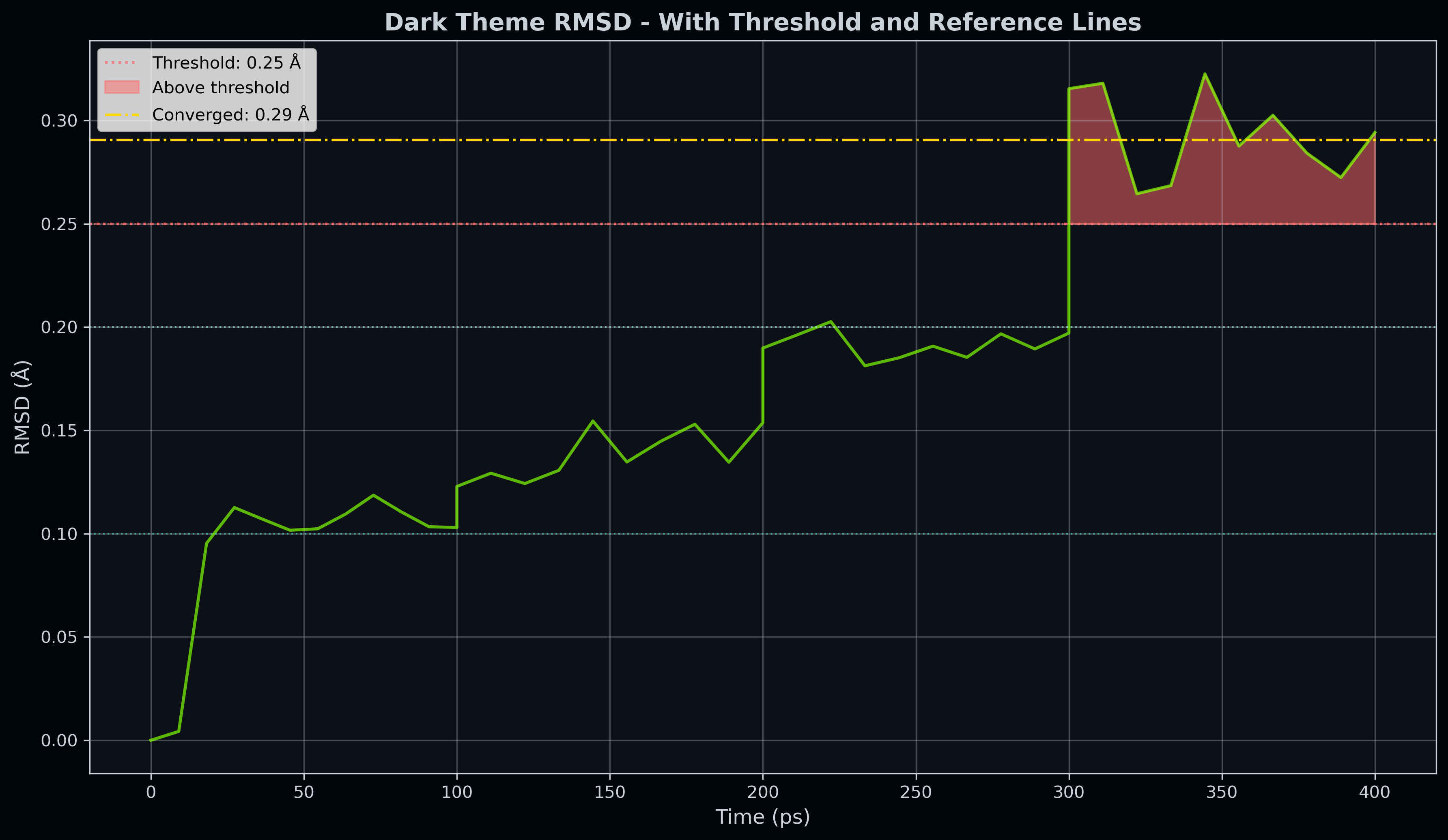
Figure: Dark theme RMSD with lines
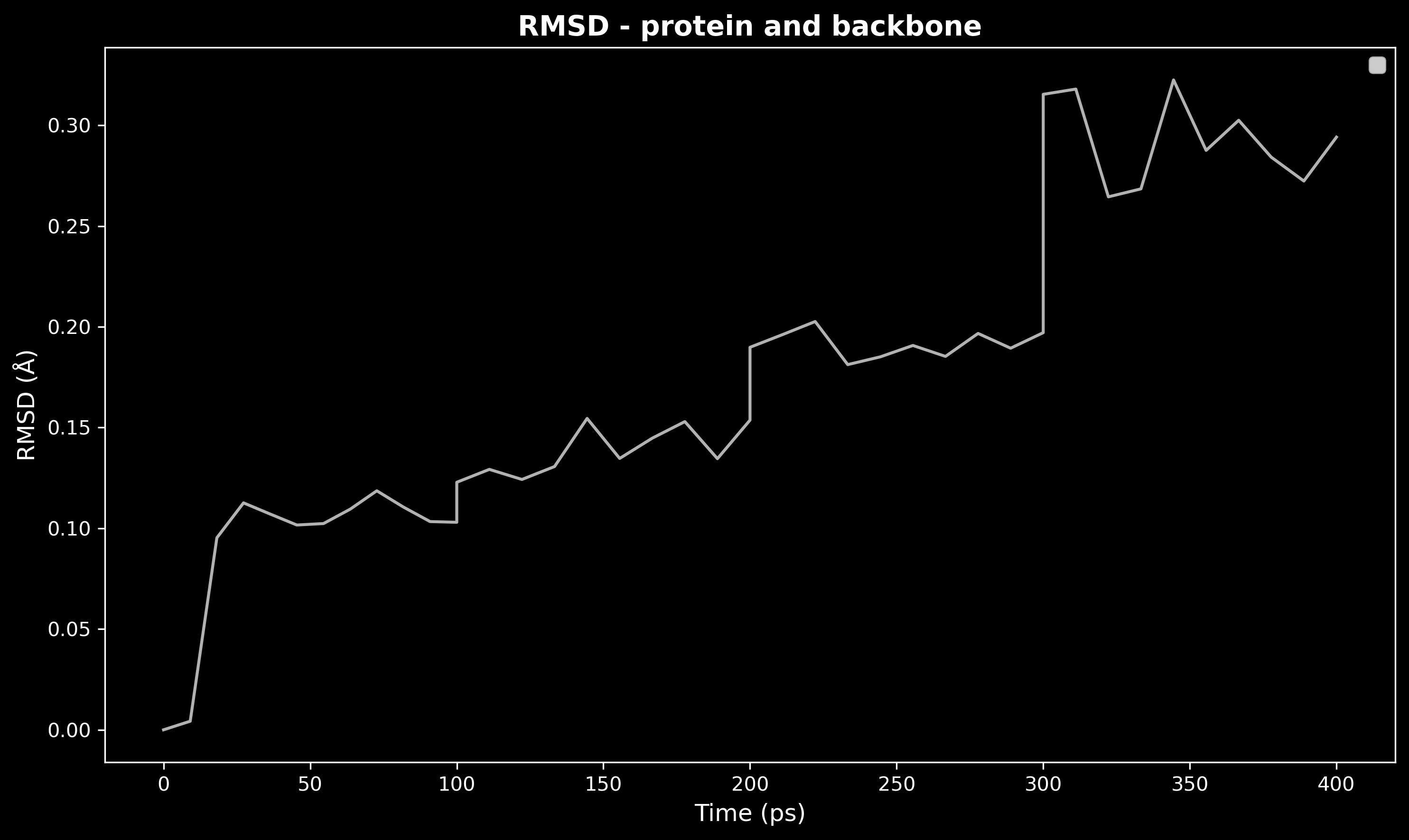
Figure: Dark theme RMSD minimal
Class: OpenMMLogAnalyzer
Parse and analyze OpenMM StateDataReporter log files. The interface mirrors EnergyAnalyzer so the two can be used interchangeably in analysis workflows.
Constructor
OpenMMLogAnalyzer(
    log_file: Union[Path, str, List[Union[Path, str]]],
    file_times: Optional[Dict[str, float]] = None,
)
| Parameter | Type | Description |
|---|---|---|
log_file | str \| Path \| list | Path to a single OpenMM log file, or a list of paths for multi-stage analysis (times are concatenated). |
file_times | dict | Optional {filename: duration_ns} mapping that overrides the time axis from the log's "Time (ps)" column. Useful when logs lack the time column or have restarted counters. |
Key differences from EnergyAnalyzer:
| Feature | EnergyAnalyzer (NAMD) | OpenMMLogAnalyzer (OpenMM) |
|---|---|---|
| Native energy units | kcal/mol | kJ/mol |
Color kwarg in plot_properties | line_colors | colors |
| Log format | space-delimited .log | tab-delimited (StateDataReporter) |
Available property keys (depend on what StateDataReporter reports):
| Key | Description |
|---|---|
potential | Potential energy (kJ/mol) |
kinetic | Kinetic energy (kJ/mol) |
total | Total energy (kJ/mol) |
temp | Temperature (K) |
volume | Box volume (nm³) |
density | Density (g/mL) |
Method: get_statistics()
Returns mean / std / min / max / initial / final for every numeric column that contains data.
Returns {key: {"mean", "std", "min", "max", "initial", "final"}}
Method: plot_energy()
analyzer.plot_energy(
    energy_units: str = "kJ/mol",
    time_units: str = "ns",
    bg_color: str = "#2b2b2b",
    fig_bg_color: str = "#212121",
    text_color: str = "Auto",
    show_grid: bool = True,
    title: Optional[str] = None,
    target_temperature: Optional[float] = None,
    target_pressure: Optional[float] = None,
    save: Optional[str] = None,
    show: bool = False,
    figsize: tuple = (12, 10),
    dpi: int = 300,
)
2×2 energy summary plot — total energy, potential + kinetic, temperature, volume / density.
| Parameter | Default | Description |
|---|---|---|
energy_units | 'kJ/mol' | 'kJ/mol' or 'kcal/mol' |
time_units | 'ns' | 'ps', 'ns', or 'µs' |
target_temperature | None | Reference temperature (K) drawn as a horizontal dashed line |
save | None | Filename for saved figure |
show | False | Display interactively |
Method: plot_properties()
analyzer.plot_properties(
    properties: Optional[List[str]] = None,
    energy_units: str = "kJ/mol",
    time_units: str = "ns",
    bg_color: str = "#2b2b2b",
    fig_bg_color: str = "#212121",
    text_color: str = "Auto",
    show_grid: bool = True,
    separate_plots: bool = False,
    save: Optional[str] = None,
    show: bool = False,
    figsize: Optional[tuple] = None,
    dpi: int = 300,
    xlim: Optional[tuple] = None,
    ylim: Optional[tuple] = None,
    colors: Optional[List[str]] = None,
)
Plot selected properties vs time. If properties is not provided, all non-empty numeric columns are plotted automatically.
| Parameter | Default | Description |
|---|---|---|
properties | None (all) | List of keys to plot, e.g. ["potential", "temp", "volume"] |
energy_units | 'kJ/mol' | 'kJ/mol' or 'kcal/mol' |
separate_plots | False | Save/show each property as its own figure |
colors | None | Line color list (one per property). Unlike EnergyAnalyzer, the kwarg is colors, not line_colors. |
save | None | Filename (or prefix when separate_plots=True) |
show | False | Display interactively |
Example 11: Basic Energy Analysis
from pathlib import Path
from gatewizard.utils.openmm_analysis import OpenMMLogAnalyzer

# Get the directory where this script is located
script_dir = Path(__file__).parent
data_dir = script_dir / "equilibration_folder"

# Single OpenMM log file (StateDataReporter output)
log_file = data_dir / "step7_production.log"

# Initialize the analyzer
analyzer = OpenMMLogAnalyzer(log_file)

# ------------------------------------------------------------------
# 1. Get statistics for all properties
# ------------------------------------------------------------------
stats = analyzer.get_statistics()

for key, s in stats.items():
    print(
        f"  {key:20s}  mean={s['mean']:12.3f}  std={s['std']:10.3f}"
        f"  min={s['min']:12.3f}  max={s['max']:12.3f}"
    )
# → All values in kJ/mol (energies) or native units (temperature in K,
#   volume in nm³, density in g/mL)

# ------------------------------------------------------------------
# 2. 2×2 summary plot: total energy, potential + kinetic, temperature,
#    volume / density
# ------------------------------------------------------------------
analyzer.plot_energy(
    save="energy_summary_example_11.png",
    show=False,
    target_temperature=303.15,
)

print("Energy summary saved: energy_summary_example_11.png")

# ------------------------------------------------------------------
# 3. Same plot converted to kcal/mol
# ------------------------------------------------------------------
analyzer.plot_energy(
    energy_units="kcal/mol",
    save="energy_summary_kcal_example_11.png",
    show=False,
)

print("Energy summary (kcal/mol) saved: energy_summary_kcal_example_11.png")
Example 12: Multi-Stage Analysis
from pathlib import Path
from gatewizard.utils.openmm_analysis import OpenMMLogAnalyzer

script_dir = Path(__file__).parent
data_dir = script_dir / "equilibration_folder"

# Pass a list of log files — time axis is concatenated automatically
log_files = [
    data_dir / "step1_equilibration.log",
    data_dir / "step2_equilibration.log",
    data_dir / "step3_equilibration.log",
    data_dir / "step4_equilibration.log",
    data_dir / "step5_equilibration.log",
    data_dir / "step6_equilibration.log",
    data_dir / "step7_production.log",
]

# Provide real stage durations (ns) to override the "Time (ps)" column
# — useful when logs lack the time column or have restarted counters.
file_times = {
    "step1_equilibration.log": 0.125,
    "step2_equilibration.log": 0.125,
    "step3_equilibration.log": 0.125,
    "step4_equilibration.log": 0.25,
    "step5_equilibration.log": 0.25,
    "step6_equilibration.log": 0.5,
    "step7_production.log": 50.0,
}

analyzer = OpenMMLogAnalyzer(log_files, file_times=file_times)

# ------------------------------------------------------------------
# 1. Print key statistics
# ------------------------------------------------------------------
stats = analyzer.get_statistics()

print("=== Multi-stage OpenMM analysis ===")
for key in ("potential", "kinetic", "total", "temp", "volume", "density"):
    if key not in stats:
        continue
    s = stats[key]
    print(
        f"  {key:12s}  mean={s['mean']:12.3f}"
        f"  initial={s['initial']:12.3f}  final={s['final']:12.3f}"
    )

# ------------------------------------------------------------------
# 2. Energy summary over the full trajectory
# ------------------------------------------------------------------
analyzer.plot_energy(
    save="energy_multistage_example_12.png",
    show=False,
    title="Full equilibration + production (51.375 ns)",
    target_temperature=303.15,
)

print("Saved: energy_multistage_example_12.png")
Example 13: Custom Property Plots
from pathlib import Path
from gatewizard.utils.openmm_analysis import OpenMMLogAnalyzer

script_dir = Path(__file__).parent
data_dir = script_dir / "equilibration_folder"

log_file = data_dir / "step7_production.log"
analyzer = OpenMMLogAnalyzer(log_file)

# ------------------------------------------------------------------
# 1. Plot all available properties (auto-detected)
# ------------------------------------------------------------------
analyzer.plot_properties(
    save="all_properties_example_13.png",
    show=False,
)
print("All-properties plot saved: all_properties_example_13.png")

# ------------------------------------------------------------------
# 2. Plot only energies, converted to kcal/mol
# ------------------------------------------------------------------
analyzer.plot_properties(
    properties=["potential", "kinetic", "total"],
    energy_units="kcal/mol",
    save="energies_kcal_example_13.png",
    show=False,
    colors=["#61afef", "#98c379", "#e06c75"],
)
print("Energy plots (kcal/mol) saved: energies_kcal_example_13.png")

# ------------------------------------------------------------------
# 3. Temperature and density as separate figures
# ------------------------------------------------------------------
analyzer.plot_properties(
    properties=["temp", "density"],
    separate_plots=True,
    save="temp_density_example_13",
    show=False,
)
print("Separate figures saved: temp_density_example_13_temp.png, temp_density_example_13_density.png")
Example 14: Area per Lipid
Calculate and plot the area per lipid using lipyphilic Voronoi tessellation on the membrane-protein equilibration trajectories in equilibration_folder.
from pathlib import Path

from gatewizard.utils.namd_analysis import BilayerTrajectoryAnalyzer, run_bilayer_analysis

script_dir = Path(__file__).parent
data_dir = script_dir / "equilibration_folder"

topology_file = data_dir / "system.pdb"
trajectory_files = [
    data_dir / "step1_equilibration.dcd",
    data_dir / "step2_equilibration.dcd",
    data_dir / "step3_equilibration.dcd",
]

# POPC headgroup phosphorus atoms in the AMBER lipid parametrization
LIPID_SEL = "resname PC and name P31"

file_times = {
    "step1_equilibration.dcd": 0.1,  # 0.1 ns
    "step2_equilibration.dcd": 0.1,  # 0.1 ns
    "step3_equilibration.dcd": 0.1,  # 0.1 ns
}

# ------------------------------------------------------------------
# 1. Class API — calculate area per lipid
# ------------------------------------------------------------------
analyzer = BilayerTrajectoryAnalyzer(
    topology_file,
    trajectory_files,
    file_times=file_times,
)
data = analyzer.calculate_area_per_lipid(lipid_sel=LIPID_SEL)

mean_area = float(data["mean_area_per_lipid"].mean())
print(f"Mean area per lipid: {mean_area:.1f} Ų")
print(f"Lipids analysed: {len(data['resids'])}")
print(f"Frames analysed: {data['areas'].shape[1]}")

# ------------------------------------------------------------------
# 2. Plot mean area per lipid time series
# ------------------------------------------------------------------
analyzer.plot_area_per_lipid(
    lipid_sel=LIPID_SEL,
    series="mean",
    time_units="ns",
    save="area_per_lipid_example_14.png",
    show=False,
)
print("Plot saved: area_per_lipid_example_14.png")

# ------------------------------------------------------------------
# 3. JSON API — run_bilayer_analysis()
# ------------------------------------------------------------------
result = run_bilayer_analysis(
    topology_file,
    trajectory_files,
    analysis_type="area_per_lipid",
    lipid_sel=LIPID_SEL,
    file_times=file_times,
)
print(f"JSON API mean area: {result['stats']['mean']:.1f} Ų")
For other force fields, adjust lipid_sel to match your headgroup atoms, e.g. "name GL1 GL2 ROH" (MARTINI) or "name PO4" (all-atom CHARMM).
Example 15: Membrane Thickness
Calculate and plot bilayer thickness as the mean interleaflet headgroup distance (lipyphilic MembThickness) on the same equilibration trajectories.
from pathlib import Path

from gatewizard.utils.namd_analysis import BilayerTrajectoryAnalyzer, run_bilayer_analysis

script_dir = Path(__file__).parent
data_dir = script_dir / "equilibration_folder"

topology_file = data_dir / "system.pdb"
trajectory_files = [
    data_dir / "step1_equilibration.dcd",
    data_dir / "step2_equilibration.dcd",
    data_dir / "step3_equilibration.dcd",
]

LIPID_SEL = "resname PC and name P31"

file_times = {
    "step1_equilibration.dcd": 0.1,  # 0.1 ns
    "step2_equilibration.dcd": 0.1,  # 0.1 ns
    "step3_equilibration.dcd": 0.1,  # 0.1 ns
}

# ------------------------------------------------------------------
# 1. Class API — calculate membrane thickness
# ------------------------------------------------------------------
analyzer = BilayerTrajectoryAnalyzer(
    topology_file,
    trajectory_files,
    file_times=file_times,
)
data = analyzer.calculate_membrane_thickness(lipid_sel=LIPID_SEL)

mean_thickness = float(data["thickness"].mean())
print(f"Mean membrane thickness: {mean_thickness:.1f} Å")
print(f"Frames analysed: {len(data['thickness'])}")

# ------------------------------------------------------------------
# 2. Plot membrane thickness time series
# ------------------------------------------------------------------
analyzer.plot_membrane_thickness(
    lipid_sel=LIPID_SEL,
    time_units="ns",
    save="membrane_thickness_example_15.png",
    show=False,
)
print("Plot saved: membrane_thickness_example_15.png")

# ------------------------------------------------------------------
# 3. JSON API — run_bilayer_analysis()
# ------------------------------------------------------------------
result = run_bilayer_analysis(
    topology_file,
    trajectory_files,
    analysis_type="membrane_thickness",
    lipid_sel=LIPID_SEL,
    file_times=file_times,
)
print(f"JSON API mean thickness: {result['stats']['mean']:.1f} Å")
To exclude cholesterol from a mixed bilayer thickness calculation, pass leaflet_filter_sel="resname DPPC DOPC" and set lipid_sel to the headgroup atoms of the lipids included in the calculation.
See Also
- User Guide - Complete usage guide
- Examples - Working code examples
- Troubleshooting - Common issues